3.1.1 Measuring System Classification
Different Types of Measuring Principles
Linear distance measurement in industrial applications uses various high-precision distance measuring systems. These systems can be classified into different categories based on the physical measuring principle.
Magnetoresistive Systems
Use MR sensors or Hall effect sensors to record periodic changes in scale magnetization. Unlike optical systems, magnetic systems are not affected by dirt. Typical pitch periods are between 0.4 and 10 mm.
Optical Systems
Use sensors to scan the pitch, recording periodic changes in reflected/transmitted light brightness or phase. Can achieve extremely fine pitches with periods less than 10 µm, providing the highest resolution.
Inductive Systems
Use mechanically structured metal scales with extremely robust design. These strips work like transformer cores. Difficult to achieve pitch periods below 1mm.
Direct vs. Indirect Measurement
How the drive elements and measuring system elements work together is crucial. We distinguish between indirect measurement and direct measurement based on the principle of operation.
Indirect Measurement

Linear guideway without integral positioning measurement system
Components:
- Linear displacement converted to other measured values
- Example: Ball screw with rotary encoder
- Advantages: Low cost and compact structure
- Disadvantages: Conversion process introduces errors
Direct Measurement (MONORAIL AMS)
Linear guideway with integral positioning measurement system (MONORAIL AMS)
Components:
- Measuring system integrated in linear guideway
- More accurate readings
- Less affected by environmental factors
- Recommended for precision applications
3.1.2 Distance Measuring Principle Overview
| Distance Measuring Principle | Optical | Magnetoresistive | Inductive |
|---|---|---|---|
| Resolution | ● ● ● | ● ● ● | ● |
| Ease of integration | ● | ● ● ● | ● ● ● |
| Sensitivity to dirt | ● | ● ● | ● ● ● |
| Installation space | ● | ● ● ● | ● ● ● |
| Installation | ● ● | ● ● ● | ● ● ● |
● = Satisfactory, ● ● ● = Very good
3.1.3 Magnetoresistive Measuring Technology
Magnetoresistive Effect
All magnetoresistive effects are based on the fact that ferromagnetic thin layers change their ohmic resistance due to an external magnetic field. The sensors in SCHNEEBERGER distance measuring systems use the anisotropic magnetoresistive effect (AMR effect).
Three Known Effects
- AMR (Anisotropic Magnetoresistance) - Used by SCHNEEBERGER
- GMR (Giant Magnetoresistance)
- TMR (Tunnel Magnetoresistance)
The sensors in SCHNEEBERGER distance measuring systems use the anisotropic magnetoresistive effect (AMR effect), which was discovered by Thomson in 1857 in ferromagnetic materials. When the direction of current in a conductor is parallel to the magnetization direction, its resistance increases by a few percent compared to when the current direction is perpendicular to the magnetization direction.
Using thin layers of ferromagnetic material, it is possible to manufacture magnetic field sensors by orienting their internal magnetic field through an external magnetic field. After the external magnetic field is removed, the internal magnetic field remains oriented. This is a basic property of ferromagnetic materials.

Weiss domains orientation
Weiss Domain Orientation
Magnetic regions (Weiss domains) are oriented on the external magnetic field.
Physical Phenomenon:
- External magnetic field H⃗r acts on material
- Magnetic domains spontaneously align
- Magnetization direction affects resistance value
- Forms physical basis of magnetoresistive effect
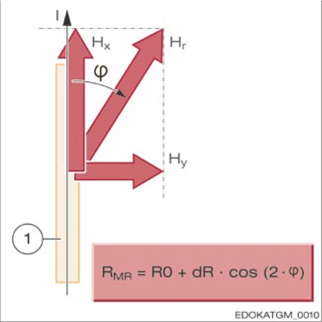
Principle of magneto-resistive sensor with MR strips
MR Strip Resistance Change Principle
Resistance Formula: RMR = R0 + dR · cos(2·φ)
MR Strip Characteristics
Magnetoresistive Incremental Sensors
Since the resistance of a single MR strip is affected by temperature changes and magnetic interference fields, four strips are typically used as sensors, configured as a Wheatstone bridge. The characteristic is that identical changes in all four resistances (e.g., due to temperature rise) do not produce a voltage difference at the output. To achieve a measurable effect, the resistances must be appropriately deflected, e.g., resistance 1 increases, 2 decreases, 3 increases, 4 decreases. This can be achieved by appropriately positioning MR strips in periodic magnetization.
It follows that each sensor is adapted to its magnetized scale period and can only be used with that period. Furthermore, MR strips are not designed individually but as series switches of multiple strips, each separated by one magnetic period. We call this equivalent positions. This allows averaging of scale variations in magnetization intensity and pole length.
Based on the quadratic characteristic curve of the sensor (measuring magnetic field strength values), an initial signal of half the magnetic scale period length can be obtained. The magnetic scale of MONORAIL AMS sensors is 400 µm, so the electrical signal period is 200 µm.
Finally, two identical structures are offset by 1/4 signal period (50 µm), thereby obtaining sine and cosine signals, which can measure the direction of motion and travel distance.
The complete schematic sensor structure is shown below:

Schematic structure of sine and cosine sensors
Component Description:
Physical Configuration:
Since both signals come from the same position on the measuring scale, this sensor is very insensitive to lateral and rotational displacement. In practice, this results in stable characteristics of periodic measurement changes. The field strength of the scale varies in the y direction from the scale. This causes the magnetic fields to cancel each other at a distance far from the scale. In the near range, at a distance of about one period length, the magnetic field strength decreases exponentially with distance in the y direction.
Magnetic Scale
SCHNEEBERGER manufactures profiled rail guideways with integrated measuring scales. Magnetic scales with periodically changing magnetic fields (N-S-N-S-N-S...) can be used with MR sensors for incremental distance measurement.

Construction of magnetic scale in profile rail
Magnetic Scale Structure:
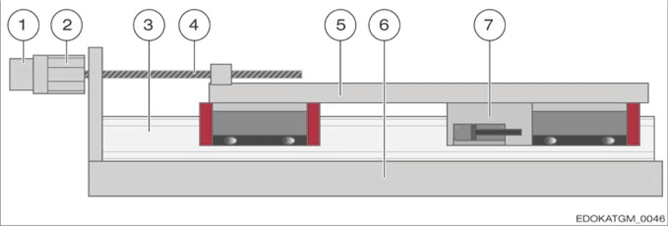
System Components
A fully functional AMS system contains:

Complete AMS measuring system components
- Guide rail with integrated measuring scale
- Accessories for mounting and connection
- Measuring carriage as complete unit
- Screws for reading head mounting
- Reading head containing sensors and electronics
The measuring carriage consists of a MONORAIL carriage with a housing mounted on one side. The housing contains a cutout with a support surface for mounting the reading head. The reading head is fastened to the housing with screws, making it easy to replace.
Contact Sampling
For correct processing of incremental signals, a consistent working distance between the sensor and measuring scale is required. Since this small tolerance cannot be achieved through rigid adjustment structures, AMS distance measuring systems use a contact sliding measurement principle.
The MR sensor is encapsulated in a shoe housing, maintained in a horizontal position by leaf springs, and pressed onto the measuring scale by compression springs. The shoe housing has ground sliding surfaces through which the constant working distance between the sensor and measuring scale is set and maintained.

Contact sampling assembly for AMS distance measuring systems
Component Description:
The shoes also form scraper edges through which larger particles and liquids cannot pass. Additionally, the scrapers of the housing mentioned above must be intact to ensure effective operating conditions for contact sampling.
This construction ensures that all wear parts and specific electronics are in the reading head. Due to the side mounting, the reading head can be replaced very easily. Small manufacturing tolerances ensure that the reading head can be easily replaced in the field while the guideway with the scale remains stationary.
3.1.4 Distance Measuring Systems
Interpolation
For distance measurement applications, interpolation refers to converting analogue input signals to digital output signals with a smaller signal period. This is necessary because counter readings and/or position readings cannot be generated directly from analogue signals.
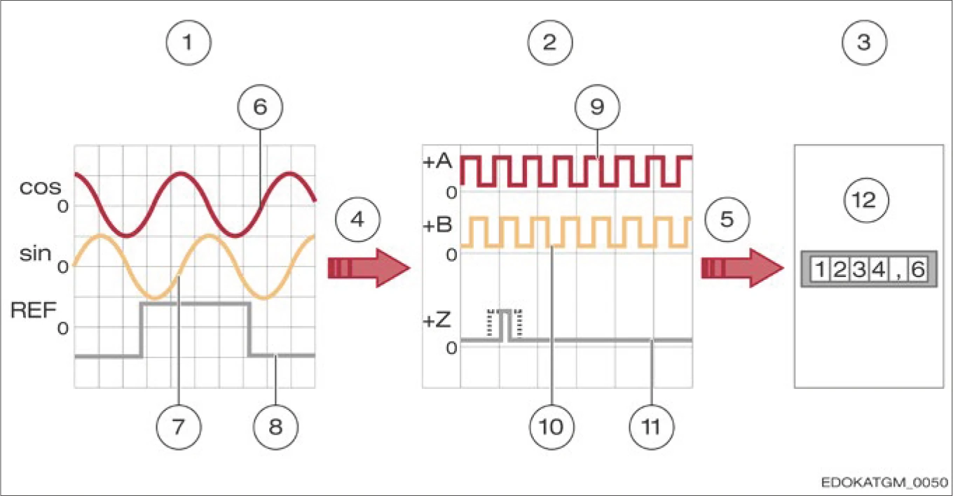
The analogue input signals (sin, cos, Ref) are interpolated (red arrow) with the digital output signals (+A, +B, +Z). Inverted signals are not represented.
For this purpose, the interpolation factor defines the signal period ratio of the analogue input signal to the digital output signal.
Signal Transmission and Evaluation
The digital signal consists of two incremental signals +A and +B and the reference signal +R, transmitted to downstream electronics. This can be a simple measuring counter, PC, or machine controller. The downstream electronics determines position values from the digital signals by counting signal edges. The counting direction is determined by the level of the related channel. Depending on how many edges are evaluated, we call it:
Single-Edge Evaluation
Only one edge of one channel is counted. One measuring step = one digital signal period.
Dual-Edge Evaluation
Rising and falling edges of one channel are counted. One measuring step = half a signal period.
Quad-Edge Evaluation
All edges of both channels are counted. One measuring step = one quarter signal period (highest resolution).

Comparison of edge evaluation methods
Amplitude Control (AGC - Automatic Gain Control)
Amplitude control refers to the function of SCHNEEBERGER AMS evaluation electronics to adjust the output amplitude to a specific value. In AMS systems, instantaneous values of sine and cosine signals are digitized, and the amplitude is calculated accordingly. The calculated value is compared with the nominal value, and the bridge voltage Ub of the MR sensor is adjusted accordingly. This results in stable voltage output values. After adjustment, new better instantaneous values are produced.
MONORAIL AMS Specifications
- Control time: Between 2 kHz and 10 kHz
- Automatically adjusts bridge voltage to maintain stable output
- Continuously optimizes signal quality
Power Sense Function
All AMS products are equipped with power sense lines (see pin layout for supply voltage feedback) to compensate for voltage drop in long power supply lines. If the controller being used supports this function, we recommend using it to guarantee reliable operation of the reading head.
Key Features
- Power sense line integrated in all AMS products
- Compensates for voltage drop in long power lines
- Improves reading head functional reliability
- Optional function (requires controller support)
Accuracy Class
The accuracy class specifies the maximum expected measurement deviation of the system under specified operating conditions. A distance measuring system with accuracy class 5 µm allows deviations of ±5 µm. For comparison purposes, accuracy class is specified based on a reference length of 1 meter.
Key Concepts
- Definition: Maximum expected measurement deviation
- Conditions: Operating under specified environmental conditions
- Example: 5 µm accuracy class = ±5 µm deviation
- Reference length: 1 meter (for specification)
Resolution
Resolution describes the smallest position change that can be measured in the measuring system. It is determined by the analogue signal period, interpolation factor, and evaluation procedure (integration time or sampling rate). For example, with an interpolation factor set to 100 and an input signal period of 200 µm, the output signal period is 2 µm, and with quad-edge evaluation in the controller, the resolution is 0.5 µm.
Resolution Calculation
- Depends on: Analogue signal period × Interpolation factor × Evaluation method
- Example: 200 µm signal × 100 interpolation = 2 µm output signal
- Quad-edge evaluation: 2 µm ÷ 4 = 0.5 µm resolution
Sampling Rate
Sampling rate describes the frequency at which the analogue signal is sampled per time interval. Usually the time interval is one second, so the unit of sampling rate is Hz. According to the Nyquist-Shannon theorem, the sampling frequency should be at least twice the original signal frequency to guarantee approximately complete reproduction of the original signal.
Key Principles
- Defined as: Frequency per time interval
- Standard unit: Hz (samples per second)
- Nyquist-Shannon theorem: Sampling frequency ≥ 2 × Signal frequency
- Ensures: Accurate signal reproduction
Reversal Error/Hysteresis
If repeated positioning accuracy measurements are made alternately in opposite directions using an appropriate test setup in each case, the average position difference of the distance measuring system between approach from the right and approach from the left can be found. This difference is called reversal error or hysteresis. SCHNEEBERGER specifies this value in its technical data sheets. Unidirectional repeatability is usually significantly lower than the specified hysteresis value.
Repeatability
The unidirectional repeatability of a measuring system is generally understood as the ability of a specific system to repeat results under exactly the same environmental conditions. In this evaluation, the measurement error must be known and included in the analysis. The repeatability of a machine tool can be determined using simple methods for a specific position and a specific direction of travel. In evaluating repeatability, many measurements are completed, and the arithmetic mean and standard deviation are calculated.

Hysteresis and repeatability measurement diagram
Measurement Diagram:
Referencing
Incremental measuring systems (such as AMS-3B and AMS-4B) cannot determine absolute position after power-on, so another magnetic track is added to the incremental track, namely the reference track. Individual reference points, reference point grids, or distance-coded reference points can be set on this reference track. A reference move is required to reference the system.
The counter can then use the reference signal to modify the internal counter to a specified value. In this process, the counter recognizes predefined positions of the incremental signals relative to each other, which is usually SIN = COS and both greater than zero, as additional information REF = "high". The following figure shows the inverted signal path, which means the negative values of the signals are illustrated.

Reference signal interfaces (analogue voltage)
Reference Signal Identification
- SIN = COS Signal relationship
- Both signals greater than zero
- REF signal = "high"
- Reference move required to establish position
- Analogue voltage interface: TSU/TRU/TMI
- Signal period: 200 µm
Individual Reference Point
An individual reference point represents the simplest function of the reference track, which can be set at any position on the scale. At SCHNEEBERGER, a reference point consists of three magnetic reference markers, which are sampled using a separate MR bridge without averaging. One reference datum represents the rising edge of the reference pulse, another the falling edge. The third reference datum is redundant, used to improve the operational reliability of the reference point identification system.
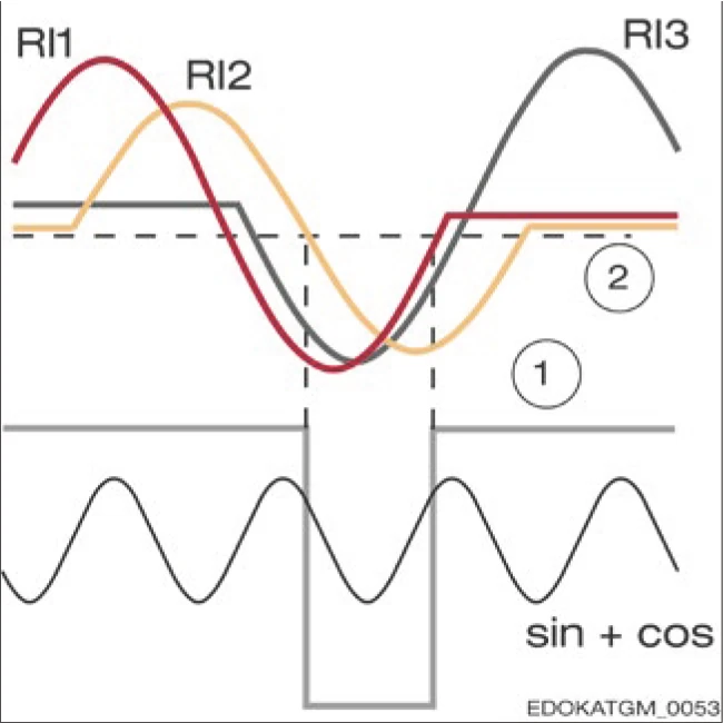
Reference point identification system
System Components:
Reference Point Grid
In the case of a reference point grid, multiple reference points are set at equal distances along the scale. The customer selects one of these reference points for referencing the axis.
Compared to individual reference points, the advantages of grids are first shortening the reference stroke by targeted application of external additional elements (cams, proximity switches, etc.), but also the ability to operate multiple measuring carriages on one guideway. For this purpose, individual reference points along the scale are assigned to different measuring carriages for the relevant reference.
Advantages over Individual Reference Points
- Reduced reference stroke distance
- Multi-carriage support capability
- Flexible selection options
- Better integration with machine automation
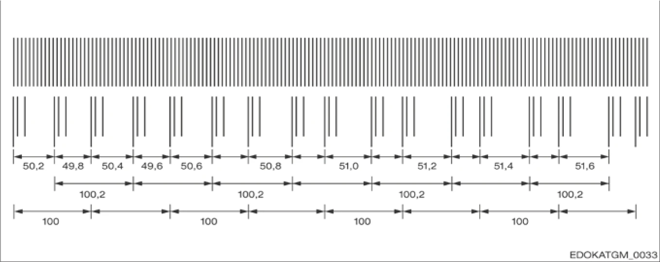
Distance Coding
In the case of distance-coded reference points, they are arranged on the scale so that each spacing between two reference points occurs only once. For example, if you cross three reference points on a distance measuring system guideway, the controller can calculate the absolute position. This represents an industrial standard supported by many controller manufacturers.
The value 100 is usually specified as the base period, representing the distance that needs to be traveled in the worst case to complete the reference. The base period determines the maximum encodable length. For short axes, it is wise to select a smaller base period to reduce the maximum necessary travel distance.
Therefore, SCHNEEBERGER offers customer-specific distance-coded reference points with different base periods for its AMS products.
Distance coding principle diagram
Absolute Coding
For absolute measuring systems, a track with absolute coding is used instead of a reference track. This coding system is either applied serially on one track or in parallel on multiple tracks. Theoretically, it should be possible to measure distance using only this track, but since the resolution of this code is relatively small, absolute coding tracks are usually combined with incremental tracks. Therefore, the absolute code defines the signal period in which the measuring system is located, and fine resolution within that signal period is obtained by interpolating the incremental signal.
The following graphics provide examples of coding systems:
Serial-coded
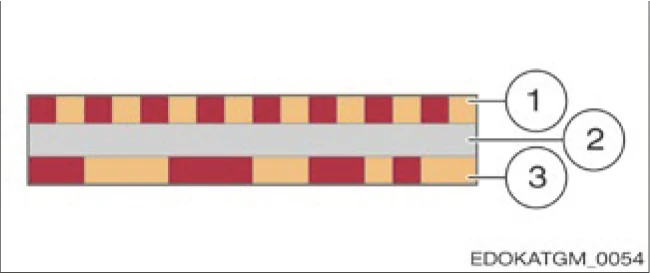
Serial-coded interpolation track
Component Description:
Parallel-coded
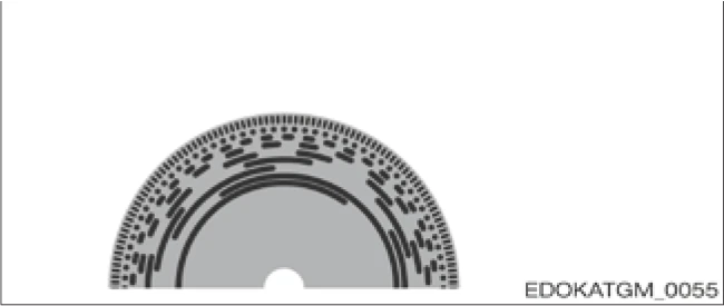
Parallel-coded pulse disc
Features:
In the case of serial-coded tracks, absolute position can only be determined by comparing two consecutive signal periods. Therefore, despite the fact that absolute position is known, two different procedures are being used.
One possibility is to use sensors that are correspondingly long so that they cover the necessary code to determine absolute position. Therefore, they are able to determine absolute position directly at any position.
Another possibility is to construct the evaluation electronics on a two-channel basis. Even when the machine is turned off, one of the channels always operates (battery-buffered) and determines any position change of the axis. When the machine is turned on, this low-resolution position information is combined with high-resolution position information from the other channel to achieve correct absolute position.
SCHNEEBERGER uses battery-buffered scanning for absolute position determination. For this purpose, a special distance-coded reference track is applied to the guideway as an absolute track. The measuring system determines the distance between three adjacent reference markers during this process and determines the instantaneous absolute position by matching the determined values with a stored matrix. In this example, the reading head passes through three reference markers and determines their spacing "1" (Code Y) and "5" (Code X). The absolute position "Pos 1:5" can then be assigned to these two measured values in a two-dimensional matrix.

Example for determining position by means of battery-buffered scanning
Diagram Components:
One-dimensional Distance Measuring Deviation
Two-dimensional Matrix
| Code Y/Code X | 1 | 2 | 3 | 4 | 5 | ... |
|---|---|---|---|---|---|---|
| 1 | Pos 1;1 | Pos 1;2 | Pos 1;3 | Pos 1;4 | Pos 1;5 | ... |
| 2 | Pos 2;1 | Pos 2;2 | Pos 2;3 | Pos 2;4 | Pos 2;5 | ... |
| 3 | Pos 3;1 | Pos 3;2 | Pos 3;3 | Pos 3;4 | Pos 3;5 | ... |
| 4 | Pos 4;1 | Pos 4;2 | Pos 4;3 | Pos 4;4 | Pos 4;5 | ... |
| 5 | Pos 5;1 | Pos 5;2 | Pos 5;3 | Pos 5;4 | Pos 5;5 | ... |
| ... | ... | ... | ... | ... | ... | Pos Y;X |
To qualify measuring scales, SCHNEEBERGER uses procedures supporting "VDI/VDE 2617 Guideline for checking distance measurement using DIN EN ISO 10360-2". In this process, the focus is on obtaining the highest possible benefit for the customer in terms of technical specifications. Technical data uses three different distance measuring deviation specifications:
- Periodic deviation
- Distance measuring deviation over a 40 mm route
- Distance measuring deviation over a 1 m route
To safeguard scale quality, limit curves for allowable deviations are established. Limit curves and measurement deviations for different reference lengths commonly used by customers are listed in the charts.
Therefore, interpolation between the specifications of SCHNEEBERGER measuring systems is allowed.
Periodic Deviations
All incremental distance measuring systems are accompanied by the effect of periodic deviations whose wavelength corresponds exactly to the scale pitch or fractions of the scale pitch. This periodic deviation or short-wave deviation is caused by small deviations in the sensor or electrical signal processing. Sine and cosine signals therefore deviate from mathematically exact form. Deviations can be classified according to arrangement (harmonics).
| KWF Period | Deviation occurs due to |
|---|---|
| 1 signal period | Sine/cosine offset |
| 1/2 signal period | Sine and cosine amplitude are different |
| 1/3 - 1/8 signal period | Sensors deliver a signal fundamentally different from sine wave shape |
Interpolation Error
If periodic deviation only occurs during digitization and position calculation, we call it interpolation error. In some cases, this can easily occur when emitter and receiver circuits are not precisely matched to each other.
Comparator Error / Abbe Error
Comparator error, also called Abbe error, is a systematic deviation that occurs when the axis of the length standard and the axis of the distance standard are not coincident. The cause of deviation is small rotational movements in axis design, which affect measurement results.
Absolute Position Determination Method Summary
1. Sensor-based Method:
- Long sensors cover necessary code
- Directly determine absolute position
- No sequential period comparison needed
2. Two-channel Battery-buffered Method:
- One channel always operates (battery-buffered)
- Second channel high-resolution when powered
- Position tracking capability when machine is off
- Combines low and high resolution at machine startup