Linear Drive Advantages
Performance
- No motion conversion required
- The drive system has no elasticity, backlash, friction, or hysteresis caused by transmission or coupling elements.
- Compact motor
- Due to the high feed force relative to low accelerated mass, extremely high acceleration performance is achievable. The full range from zero speed to maximum speed is usable.
- Direct position measurement
- Through direct position measurement and a rigid mechanical structure, the positioning process is highly dynamic and precise.
Operating Costs
- No additional moving parts
- Assembly, adjustment, and maintenance work for drive components is significantly reduced.
- No wear in the drive system
- Even under high alternating loads, the drive system is extremely durable. Machine downtime is thus significantly reduced.
- High availability
- In addition to extended service life and reduced wear, the robustness of linear motors also improves system availability.
- Mechanical overload in the drive system does not cause damage as it would with geared motors.
Design
- Compact installation space
- The compact design reduces the space requirements of the drive module.
- Fewer components
- The proven design facilitates the integration of motor components into the overall machine concept.
- Fewer and more robust components result in a low failure rate (high MTBF*).
- Diverse design variants
- Facilitates optimal integration of motor components into the overall machine design concept.
*MTBF: Mean Time Between Failures
Linear Motor Characteristics
Linear drives enable linear motion without the need for motion converters or intermediate gears.
A linear motor consists of a primary part and a secondary part. The primary part contains the winding coils, and the secondary part consists of a set of permanent magnets arranged opposite the primary part. Motor types can be classified as slotted, slotless, and ironless, as well as stepper motors (synchronous reluctance hybrid motors).
The motor produces uniform and typical force within a specific speed range. The magnitude of the force is determined by the effective air gap area between the primary part and the secondary part.
When current is applied to the primary part, the electromagnetic field around the winding coils generates a force acting on the secondary part, producing linear motion.
A linear axis system requires an appropriate guidance system to maintain the air gap between the primary part and the secondary part, as well as a linear measurement system to detect the motor position.
Each motor series includes selections of different lengths and widths to meet various force and installation requirements, and offers multiple mounting and connection variants.
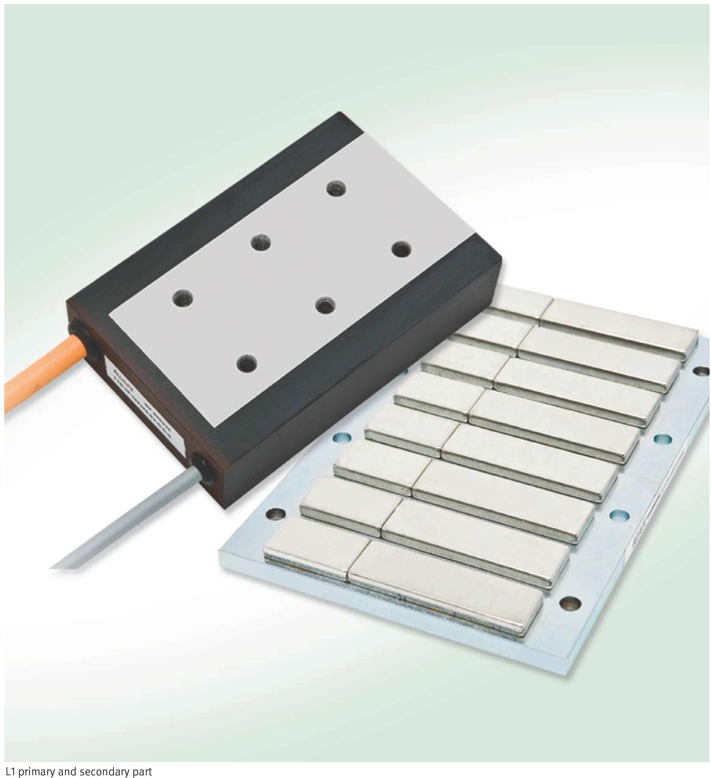
L1 Linear Motor: Primary Part and Secondary Part
Linear Motor Series Overview
Slotted Motors
| Motor Type | Characteristics |
|---|---|
| L1A Series | Peak force up to 1010 N | Outstanding force-to-weight ratio | Suitable for automation applications with limited vertical installation space |
| L1B Series | Peak force up to 1521 N | Optimized thermal dissipation | Suitable for automation applications requiring higher feed forces |
| L1C Series | Peak force up to 5171 N | Optimized thermal dissipation | Water cooling | Suitable for machine tool applications |
| L2U Series | Peak force up to 12000 N | Double comb structure | Outstanding force-to-volume ratio | Long service life / High dynamic performance | Cooling options | Constant velocity | Magnetic attraction force neutralization | Suitable for machine tool applications |
Low-Iron Motors / Slotless
| Motor Type | Characteristics |
|---|---|
| FSM Series | Flat design | Minimized ripple force | High dynamic performance and high precision | Suitable for measuring machine applications |
Ironless Motors
| Motor Type | Characteristics |
|---|---|
| ULIM Series | Excellent dynamic performance | Constant velocity | Compact design | Suitable for printing machines and product electronics applications |
Reluctance Motors
| Motor Type | Characteristics |
|---|---|
| LRAM | Stepper motor | Wear-free | Precision air bearing | Suitable for pick-and-place applications in product electronics | Suitable for low-mass applications |
Motor Parameters — Efficiency Criteria
Based on the motor size, the power losses (copper losses) generated by force and process at different operating points are fixed and independent of winding design. Since linear motors do not output mechanical power at standstill, it is not meaningful to cite an efficiency coefficient here.
Power Loss Formula
When current is converted to holding or feed force, power losses or heating proportional to the square of the load-independent current are generated. This relationship holds in the linear dynamic range and under static operation at room temperature.
Pl = (F / km)2
- Pl: Power loss [W]
- F: Force [N]
- km: Motor constant [N/√W]
The motor constant km can be used as a means of comparing the efficiency of different motors. A higher motor constant represents a more efficient conversion of force relative to power loss.
km vs. Temperature
The motor constant km depends on the ohmic resistance and therefore also on the winding temperature of the motor. In motor technical data, km is referenced at 25 °C.
The figure below shows the dependence of the reference motor constant on temperature: at a winding temperature of 100 °C, km decreases to approximately 88% of its value at 25 °C.
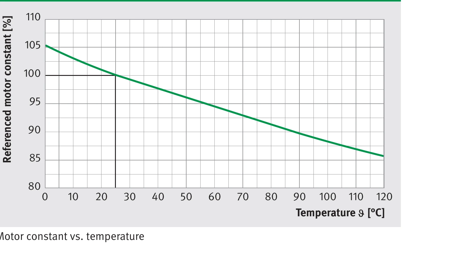
Motor constant km dependence on winding temperature (referenced to 100% at 25 °C)
High-Speed Note
As speed increases, the power loss Pl is additionally supplemented by frequency-dependent magnetic reversal losses and eddy current losses, which are not included in the motor constant km, but become significant in the limit speed range and must be taken into account. The motor constant km is only valid for the linear region of the force-current characteristic.
Winding Design and Dependencies
The achievable limit speed of any linear motor depends largely on the winding design and the DC bus voltage (UDCL). The internal voltage drop of the motor increases with speed. At the specified limit speed, the voltage demand for field-oriented control corresponds to the bus voltage of the servo converter. Beyond this point, speed drops sharply.
The higher the bus voltage, the lower the winding-related voltage constant (ku), and the higher the achievable limit speed. Due to the relationship between voltage constant and force constant, the force constant increases at higher speeds as the current demand for the same force increases.
Winding Variants
For winding data, a standard winding WM (suitable for medium dynamic requirements) is predefined for each motor size. For lower or higher dynamic requirements, winding variants WL and WH are additionally available.
- WL: Low dynamic requirements (limit speed at lower bus voltage decreases approximately proportionally)
- WM: Standard dynamic requirements (default winding)
- WH: High dynamic requirements
The force-current characteristic describes the force at different operating points. The force-speed characteristic shows the relationship between force and speed at different operating points.
L1 Linear Motor Series
Force-Speed Characteristics
The F(v) characteristic of a permanent magnet synchronous motor is nearly independent of speed in the low-speed range. This applies to Fp, Fcw, and Fc up to their corresponding corner speeds vlp, vlcw, and vlc. At higher speeds, the force gradually decreases due to the effect of back EMF*, ultimately dropping to zero.
Higher bus voltages compensate for larger back EMF, allowing higher speeds to be reached.
Operating Conditions
The motor can operate at any operating point below the F(v) characteristic curve:
- In uncooled continuous operation, force can reach up to Fc
- In water-cooled continuous operation, force can reach up to Fcw
- In cyclic intermittent operation (S3**), force can reach up to Fp
For closed-loop controlled motor motion, an appropriate margin must be maintained between the potential operating point and the declining region of the F(v) characteristic. A margin of approximately 0.2 times the maximum speed is typically reserved as control reserve.
Force at v = 0 m/s
When using continuous force (Fs) at standstill (e.g., Z-axis without mass compensation), note that a maximum of only 70% of the rated force may be used. Exceeding this derating value may cause local motor overload.
Fs = 0.7 × Fc (or Fcw)
*Back EMF: Back Electromagnetic Force
**S3: Operating mode per VDE 0530 standard
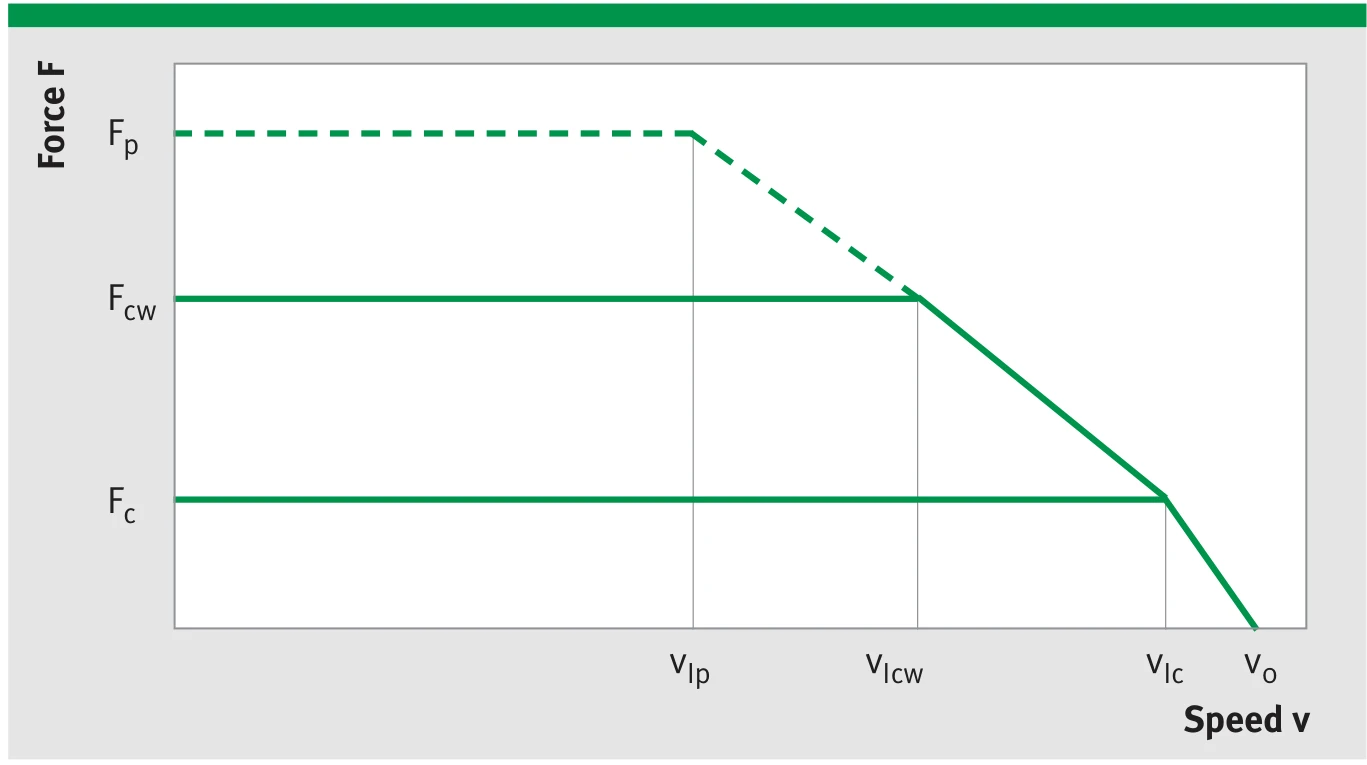
Force-Speed (F-v) characteristic: Fp (peak force), Fcw (water-cooled continuous force), Fc (uncooled continuous force) and their corresponding corner speeds
Force-Current Characteristics
The characteristic curve from the origin (0,0) to (Fpl, Ipl) is approximately linear, defined by the force constant kf:
F = I × kf
The operating point for uncooled operation (Fc, Ic) and the operating point for water-cooled operation (Fcw, Icw) both lie within this linear region.
Saturation Region
At high currents, the non-linearity of the force-current characteristic results from saturation of the motor's magnetic circuit. This segment of the curve is described in data sheets and diagrams by the force-current operating points (Fp, Ip) and (Fu, Iu), with a slope much flatter than kf.
The motor can operate at the operating point (Fp, Ip) for short periods (cyclically for ≤3 seconds), provided that the average thermal losses have been taken into account. For acceleration processes, this is the maximum operating point to be used.
Limit Point (Fu, Iu)
The limit point must never be exceeded; otherwise there is a risk of motor overload. This point is only used for short-circuit braking considerations and must not be used as a selection basis.
All parameters are explained in the glossary.
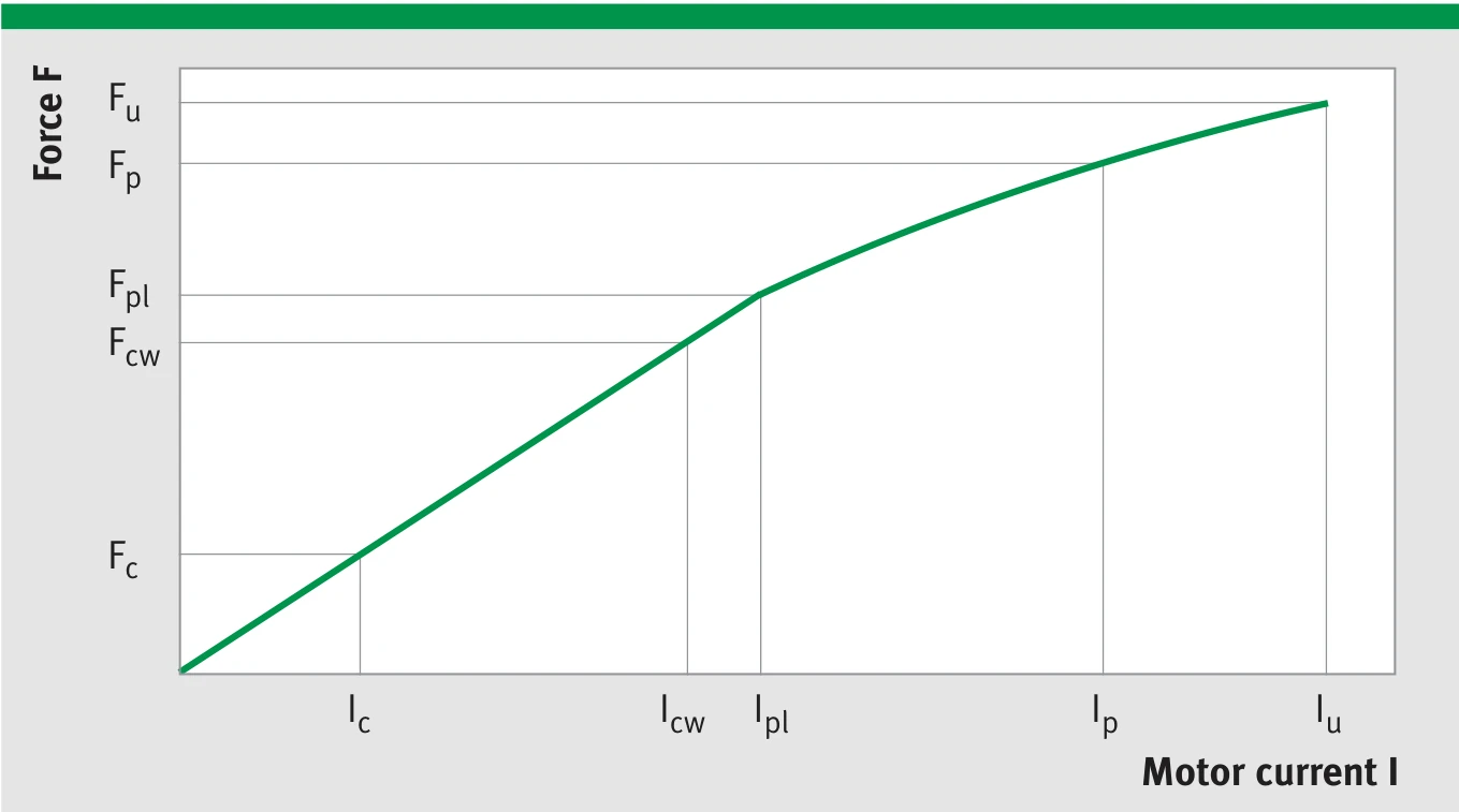
Force-Current (F-I) characteristic: linear region (defined by kf) and saturation region (Fp/Fu operating points)
Thermal Protection
Linear drives are often operated near their thermal performance limits. In addition, unforeseen overloads may occur during operation, causing the current to exceed the allowable rated current. Therefore, the servo controller for the motor should generally be equipped with overload protection to control the motor current. It must be ensured that the RMS value of the motor current is only allowed to exceed the permissible rated current for a short period. This indirect temperature monitoring is both fast and reliable.
IDAM motors are equipped with temperature sensors (PTC and KTY) that can be used for thermal protection.
Monitoring Circuit I — PTC Sensor
Each of the three phase windings is equipped with a series-connected PTC (Positive Temperature Coefficient thermistor) to ensure motor protection. The PTC is a positive temperature coefficient thermistor, and once installed its thermal time constant is less than 5 seconds.
PTC Operating Principle
When the nominal response temperature Tn is exceeded, the resistance of the PTC rises sharply, increasing to several times the cold-state value. When three PTC elements are connected in series, even if only one element exceeds Tn, the overall resistance shows a significant change.
Using three sensors ensures that a safe shutdown signal is issued even when there is asymmetric phase loading with the motor at standstill.
A commercially available motor protection trip device is connected downstream, typically triggering between 1.5 kΩ and 3.5 kΩ. In this way, overtemperature can be detected within a few degrees of each winding.
The trip device also responds when the PTC circuit resistance is too low, which usually indicates a defect in the monitoring circuit. This also ensures electrical isolation between the controller and the motor sensors. The motor protection trip device is not included in the scope of supply.
Principle: The PTC sensor signal must be monitored to protect the motor from overtemperature damage.
PTCs are not suitable for temperature measurement. If temperature measurement is required, KTY sensors should be used.
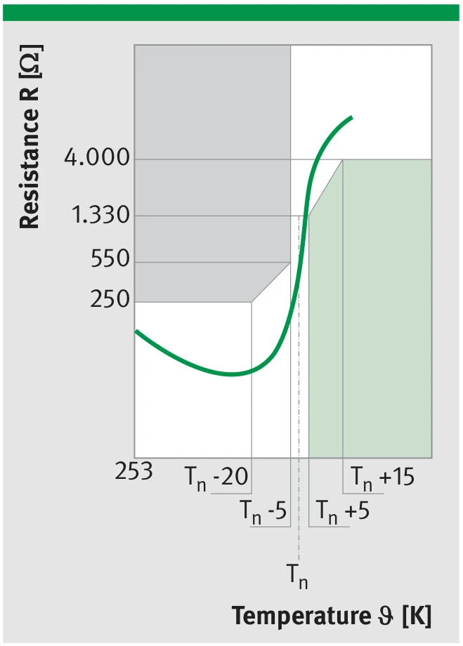
PTC sensor resistance-temperature characteristic: resistance rises sharply above nominal response temperature Tn
Monitoring Circuit II — KTY84-130 Sensor
One of the motor phases is additionally equipped with a KTY84-130 sensor. This is a semiconductor resistor with a positive temperature coefficient that produces a temperature-equivalent signal (with a delay that depends on the motor type).
To protect the motor from overtemperature, a shutdown threshold is set in the controller. When the motor is at standstill, a constant current flows through the windings, the magnitude of which depends on the respective pole position. Therefore, the motor does not heat uniformly, which may lead to overheating of unmonitored windings.
KTY Sensor Purpose
The KTY sensor monitors a single winding. Its signal can be used to observe temperature or issue a warning. It is not permitted to use KTY alone as the basis for shutdown.
Imax = 2 mA
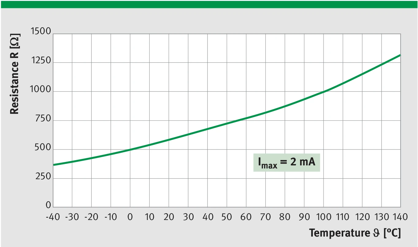
KTY84-130 sensor resistance-temperature characteristic: linear positive temperature coefficient for precise winding temperature measurement
Standard Connection of PTC and KTY
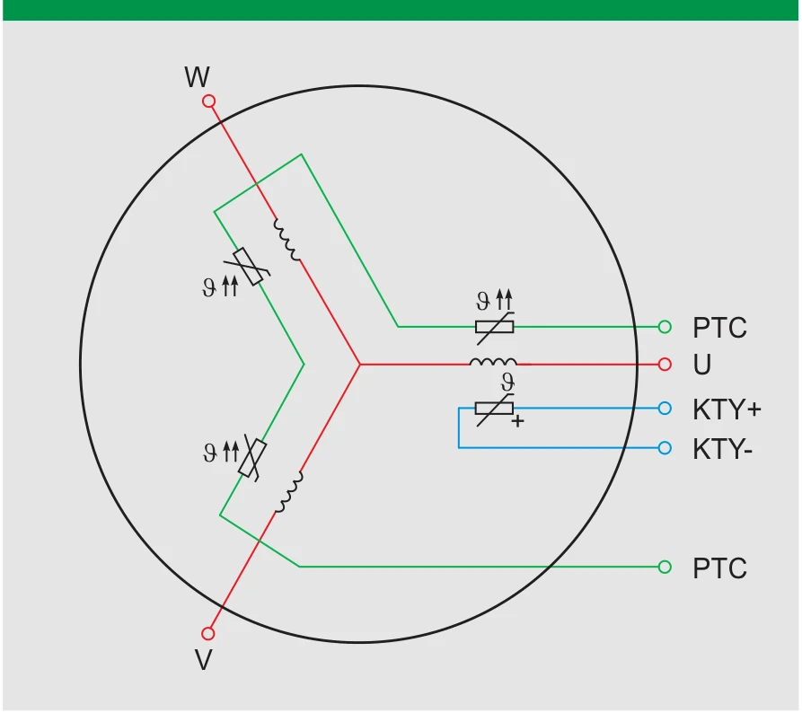
Standard connection of PTC and KTY: PTC sensors connected in series within all three-phase windings; KTY sensor connected to one winding
The PTC and KTY sensors have basic insulation and are not suitable for direct connection to PELV/SELV circuits (per DIN EN 50178 standard).
Additional monitoring sensors can be integrated at customer request.
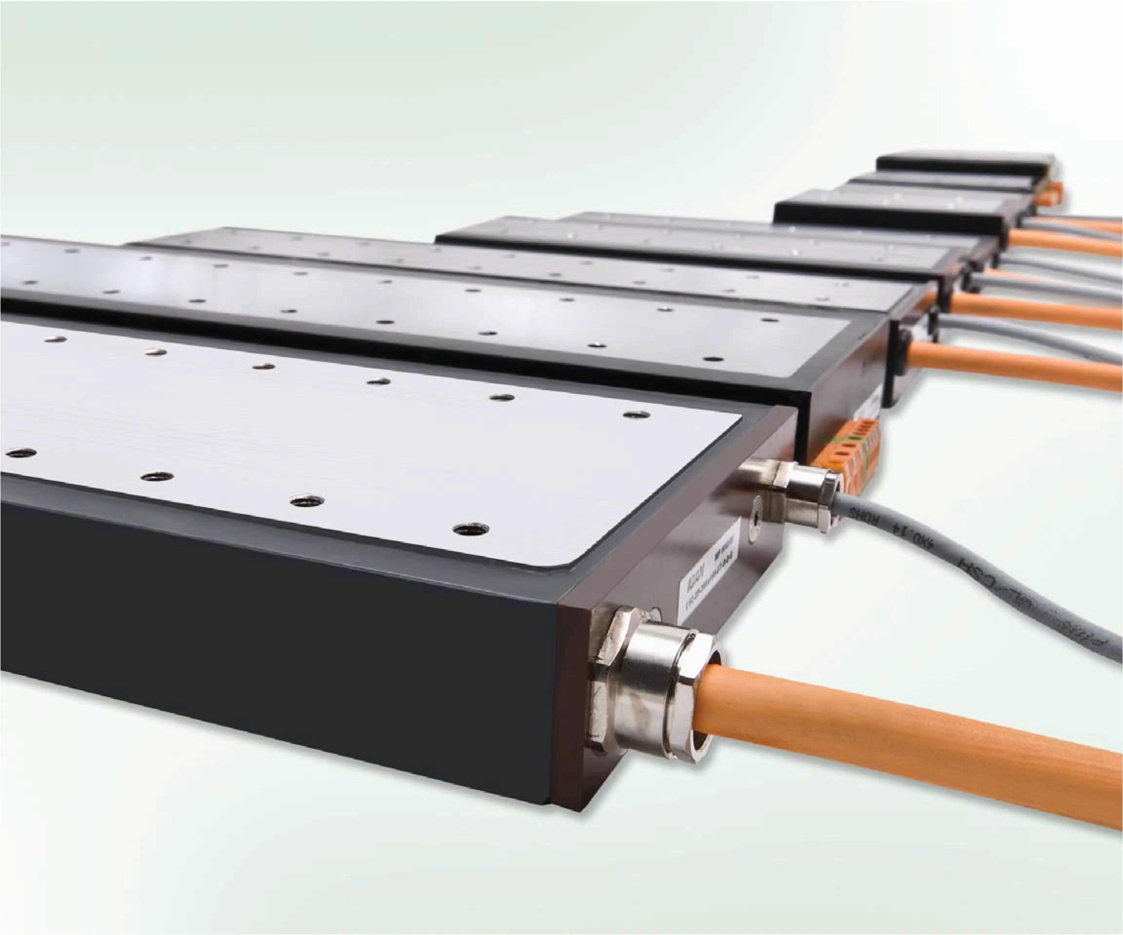
Electrical Connections
The standard connection for IDAM motors exits from the end face. The standard cable length from the cable exit point on the motor is 1000 mm. Different lengths can be provided on request. The cross-section of the power cable depends on the continuous motor current and is documented in the catalog drawings. As standard, L1A and L1B are dimensioned for the natural-cooling continuous current Ic at power loss Pl, while L1C is dimensioned for the water-cooled continuous current Icw at power loss Plcw.
The motor cable cross-section starts from 4G0.75 mm². The sensor cable 4 × 0.14 mm² (d = 5.1 mm) allows temperature monitoring via PTC and KTY. The cable ends are open with end sleeves. The cables used are UL certified and suitable for cable carriers.
A motor version with terminals (WAGO Series 236 terminal block, suitable for up to 1.5 mm² wire cross-section) is available as an alternative to end sleeves. The position of the cable outlet or terminal is indicated in the data sheets. For variants without water cooling and with continuous current not exceeding 16 A, terminal use is unrestricted.
Terminal Assignment
Motor Terminals
| Core | Terminal No. | Function |
|---|---|---|
| U | 1 | Phase U |
| VV | 2 | Phase V |
| WWW | 3 | Phase W |
| GNYE | 4 | PE (Protective Earth) |
| BK | — | Shield |
Sensor Terminals
| Core | Terminal No. | Function |
|---|---|---|
| WH | 7 | PTC |
| BN | 8 | PTC |
| GN | 5 | + KTY |
| YE | 6 | - KTY |
Positive Direction of Motion
In all three-phase motors, the electrically positive direction of motion corresponds to a clockwise rotating field, i.e., the phase voltages are induced in the sequence U, V, W. For IDAM motors, the positive direction of motion is:
- Towards the side without cable (cable version)
- Towards the side without terminal (terminal version)
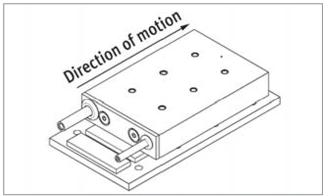
Cable version: positive direction is towards the side without cable
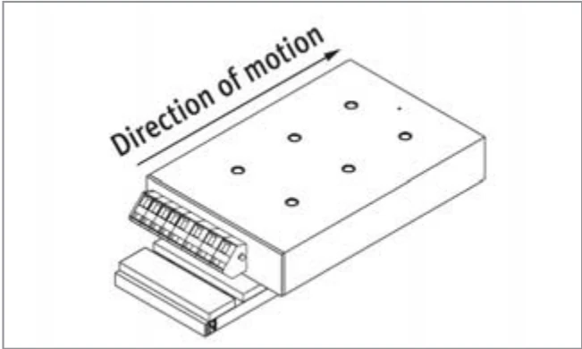
Terminal version: positive direction is towards the side without terminal
Motor Cable Selection
| Continuous Current I [A] | Cable Cross-Section [mm²] | Diameter dk [mm] | Dynamic Bending Radius rd [mm] | Static Bending Radius rs [mm] |
|---|---|---|---|---|
| ≤9 | 0.75 | 7.3 | 73 | 44 |
| ≤16 | 1.5 | 10 | 100 | 60 |
| ≤22 | 2.5 | 11.6 | 120 | 70 |
Commutation
Commutation operation is preferred for synchronous motors. IDAM linear motors are not equipped with Hall sensors as standard. IDAM recommends using a measurement system for commutation.
Commutation Methods
Synchronous motors detect rotor position via a measurement system (such as a linear encoder) and control the switching timing of the phase currents accordingly. Compared to the six-step commutation of Hall sensors, measurement system commutation achieves smoother sinusoidal current control, resulting in lower force ripple and higher positioning accuracy.
Insulation Resistance
Insulation Resistance for Bus Voltage Not Exceeding 600 VDC
IDAM motors comply with EC Directive 73/23/EEC and European Standards EN 50178 and EN 60204. They undergo staged high-voltage testing before delivery and are vacuum-impregnated.
Please ensure the rated operating voltage of the motor is observed.
Motor Terminal Overvoltage in Inverter Operation
Due to the high du/dt loads generated by rapidly switching power semiconductors, voltage spikes significantly higher than the actual inverter voltage may appear at the motor terminals, especially when using longer connection cables (over 5 m). This places very high loads on the motor insulation.
The du/dt value of the PWM module must not exceed 8 kV/µs. The motor connection cable should be kept as short as possible.
To protect the motor, it is recommended to always measure the inverter voltage (PWM) applied to the motor windings relative to PE using an oscilloscope in a specific configuration. Existing voltage spikes should not significantly exceed 1 kV. From approximately 2 kV, gradual insulation damage should be expected.
IDAM engineers will assist you in determining the application solution and reducing excessive voltages.
Please observe the recommendations and configuration instructions provided by the inverter manufacturer.
Cooling and Cooling Circuits
Power Losses and Thermal Losses
In addition to the power losses defined by the motor constant km, the motor is also subject to frequency-dependent losses at higher control frequencies (above 50 Hz). These losses together cause the motor and other system components to heat up.
The following rule applies for low control frequencies (<80 Hz): Motors with higher motor constant km produce lower power losses compared to comparable motors with lower km.
The power losses generated during operation are transferred through the motor assembly to the connected components. The entire system is carefully designed to control heat distribution through convection, conduction, and radiation.
For L1C motors, a cooling system can be optionally selected as an accessory to improve heat dissipation. The continuous force of a liquid-cooled motor is approximately twice that of an uncooled motor.
Active Cooling
Active cooling should be prioritized for machines operating at high performance and high dynamic conditions, as well as in corresponding high bearing load applications.
If complete thermal isolation between the motor and machine is required (e.g., to prevent thermal deformation in high-precision machinery), an additional thermal insulation layer and precision cooling are needed. The actual cooling constitutes the primary or power cooling system.
Cooling Plate
The motor cooling system is implemented in the form of a cooling plate installed between the motor and the machine table, which should be connected by the customer to the cooling circuit of a cooling device. The thermal insulation layer and cooling plate can be supplied as optional accessories for motor components or as part of the customer's machine design.
The cooling medium flows through internal copper tubes from the inlet to the outlet. The inlet and outlet connections can be distributed to two ports, with connection fittings of G 1/8 internal thread.
When using water as coolant, additives against corrosion and biological deposits must be added.
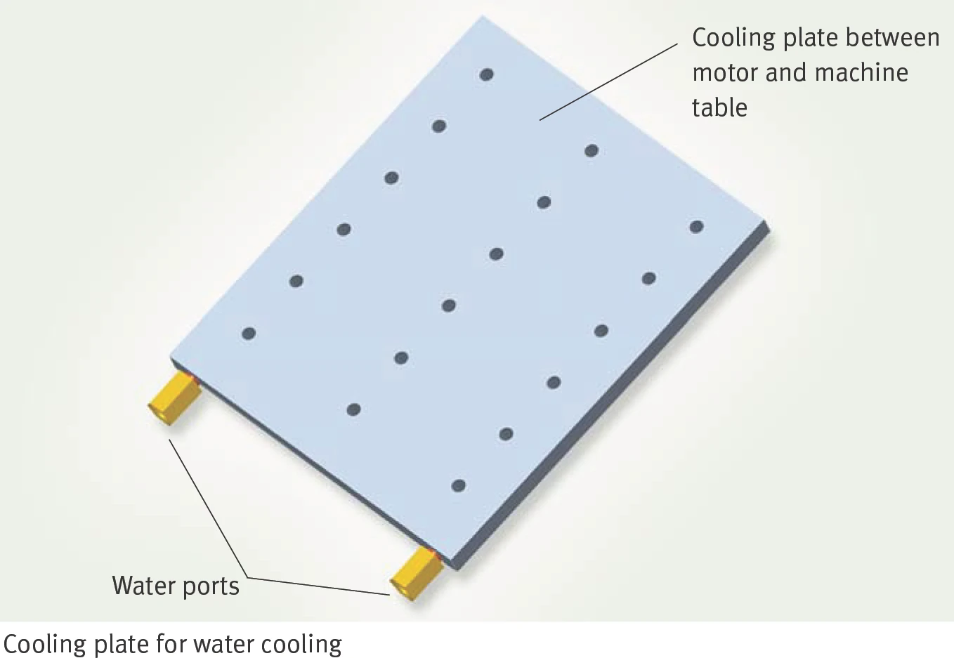
Cooling plate for water cooling
Cooling plate installed between motor and machine table
Dependency of Characteristic Data on the Supply Temperature of Cooling Medium
The continuous current Icw indicated in the data sheet for water cooled operation can be achieved at a rated supply temperature θnV of 25 °C. Higher supply temperatures θV result in a reduction of the cooling performance and therefore also the nominal current.
The reduced continuous current Ic red can be calculated by the following quadratic equation:
Ic red / Icw = √((θmax − θV) / (θmax − θnV))
- Ic red: Reduced continuous current [A]
- Icw: Continuous current, cooled at θnV [A]
- θV: Current supply temperature [°C]
- θnV: Rated supply temperature [°C]
- θmax: Maximum permissible winding temperature [°C]
(Applies to a constant motor current)
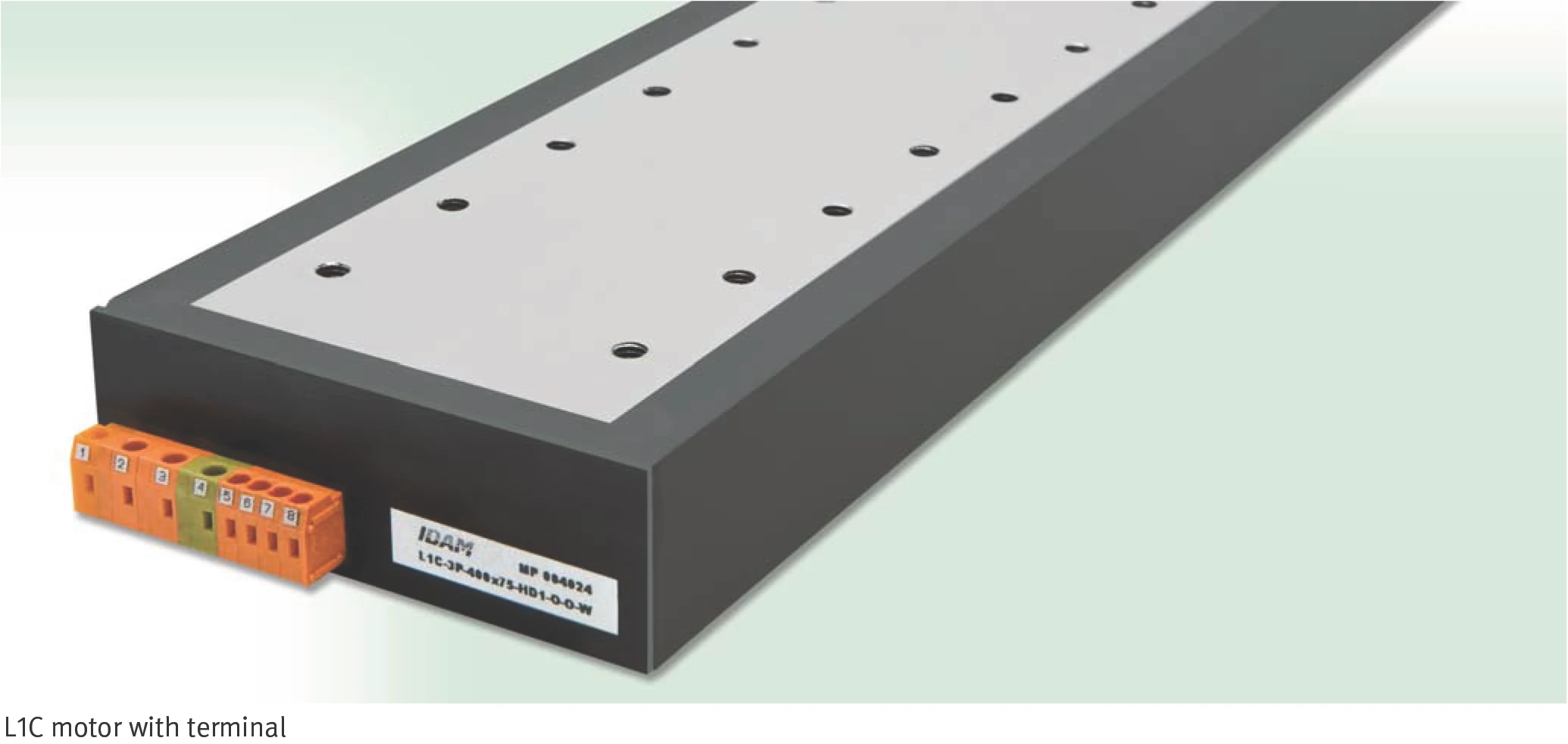
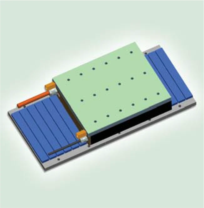
L1C motor with terminal
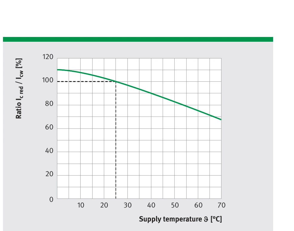
Relative continuous current Ic red / Icw vs. supply temperature θV (θnV = 25 °C)
Selection of Direct Drives for Linear Motions
Cycled Applications
In cycled operation, sequential positioning movements are interspersed with pauses during which no motion takes place. A simple positioning sequence takes the form of a positively accelerated motion followed by a deceleration (negative acceleration of usually the same magnitude, in which case acceleration and deceleration time are equal). The maximum speed vmax is reached at the end of an acceleration phase.
A cycle is described in the v(t) diagram (v: speed, t: time). The diagram shows a forward-backward movement with pauses (tM: motion time, tP: dwell time with no load).
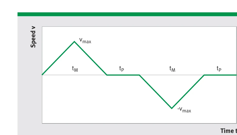
v-t diagram for cycled operation
This yields the following a(t) diagram as well as the curve for the force required for the motion:
F = m × a
- F: Force [N]
- m: Mass [kg]
- a: Acceleration [m/s²]
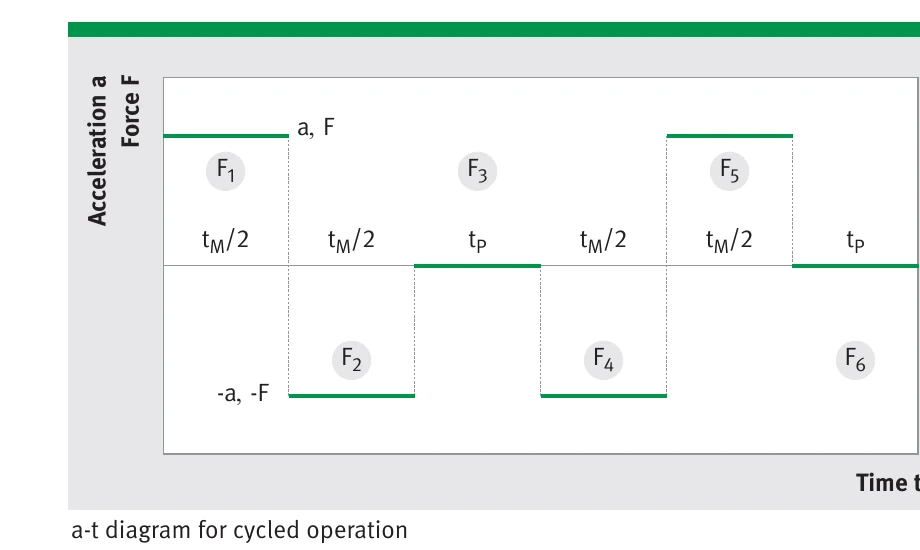
a-t diagram for cycled operation
Three Selection Criteria
The motor is selected according to three criteria in accordance with the force curve for a desired cycle:
- Maximum force: Maximum force in the cycle ≤ Fp according to the data sheet
- Effective force: Effective force in the cycle ≤ Fc (motor non cooled) or Fcw (motor water-cooled) according to the data sheet
- Maximum speed: Maximum speed in the cycle ≤ vlp according to the data sheet
Effective Force Calculation
The effective force is equal to the root mean square of the force curve (here: six force segments in the cycle):
Feff = √( (F1²·t1 + F2²·t2 + … + F6²·t6) / (t1 + t2 + … + t6) )
Using the forces F1 = F, F2 = −F, F3 = 0, F4 = −F, F5 = F, F6 = 0 and times t1 = tM/2, t2 = tM/2, t3 = tP, t4 = tM/2, t5 = tM/2, t6 = tP, this simplifies to:
Feff = F · √( tM / (tM + tP) )
This formula applies to the effective force only if all the forces acting in the cycle have the same magnitude (masses and accelerations are constant). The denominator is the cycle time (motion time + dwell time).
The safety factor 1.4 in the sample calculation also takes into account the operation of the motor in the non-linear region of the force-current characteristic, for which the formula for calculating Feff only applies approximately.
Acceleration and Maximum Speed
a = 4 · x / tM²
vmax = 2 · x / tM
- x: Total stroke [m]
- tM: Motion time [s]
- a: Acceleration [m/s²]
- vmax: Maximum speed [m/s]
The described positioning motion is performed with a (theoretically) infinite rate of jerk. If jerk limitation is programmed into the servo converter then the positioning times are extended accordingly. In this case, greater acceleration would be needed in order to maintain unchanged positioning times.
Example: Cycled Applications
| Preset Values | Calculation | ||
|---|---|---|---|
| Total stroke | x = 0.7 m | Maximum speed | vmax = 2 × 0.7 / 0.3 = 4.67 m/s |
| Mass | m = 10 kg | Acceleration | a = 4 × 0.7 / 0.3² = 31.1 m/s² |
| Motion time | tM = 0.3 s | Maximum force | Fmax = (10 kg × 31.1 m/s² + 5 N) × 1.4 = 442.4 N |
| Friction force | Ff = 5 N | Effective force | Feff = (10 kg × 31.1 m/s² × √(0.3/1.3) + 5 N) × 1.4 = 216.2 N |
| Cycle time | tcyc = 1.3 s | ||
| Safety factor | 1.4 | ||
Motor Selection — Non-Cooled
Conditions: Fmax ≤ Fp and Feff ≤ Fc
✓ L1A-3P-200-75-WM
The required speed can be achieved with a DC link voltage of 600 V.
Motor Selection — Water-Cooled
Conditions: Fmax ≤ Fp and Feff ≤ Fcw
✓ L1C-3P-100-75-WM
The cooling plate increases the accelerated mass by approx. 500 g (taken into account). The required speed can be achieved with a DC link voltage of 600 V.